In the wake of the 2015/16 El Niño, recent weeks have seen the denialoblogosphere inundated with assorted attempts to proclaim yet again that there have been “19 years without warming”. In another of his intermittent articles Great White Con guest author Bill the Frog once again proves beyond any shadow of a doubt that all the would be emperors are in actual fact wearing no clothes. Without further preamble:
Ho-hum! So here we go again. The claim has just been made that the UAH data now shows no warming for about 19 years. A couple of recently Tweeted comments on Snow White’s Great White Con blog read as follows…
For the nth time, nearly 19 years with no significant warming. Not at all what was predicted!!
and
Just calculated UAH using jan: R^2 = 0.019 It’s PROVABLE NO DISCERNIBLE TREND. You’re talking complete bollocks!!!
Before one can properly examine this “no warming in 19 years” claim, not only is it necessary to establish the actual dataset upon which the claim is based, but one must also establish the actual period in question. A reasonable starting point within the various UAH datasets would be the Lower Troposphere product (TLT), as most of us do live in the lower troposphere – particularly at the very bottom of the lower troposphere.
However, one also has to consider which version of the TLT product is being considered. The formally released variant is Version 5.6, but Version 6 Beta 5 is the one that self-styled “climate change sceptics” have instantly and uncritically taken to their hearts.
The formally released variant (Ver 5.6) is the one currently used by NOAA’s National Centers for Environmental Information (NCEI) on their Microwave Sounding Unit climate monitoring page. As can be seen from the chart and the partial table (sorted on UAH values), the warmest seven years in the data include each of the four most recent years…
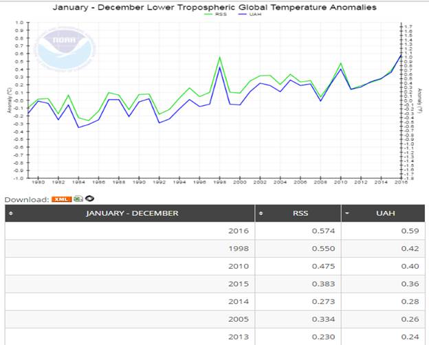
The above chart clearly doesn’t fit the bill for the “no warming in 19 years claim”, so, instead we must look to the Version 6 Beta 5 data. Before doing so, a comparison of the two versions can be quite revealing…
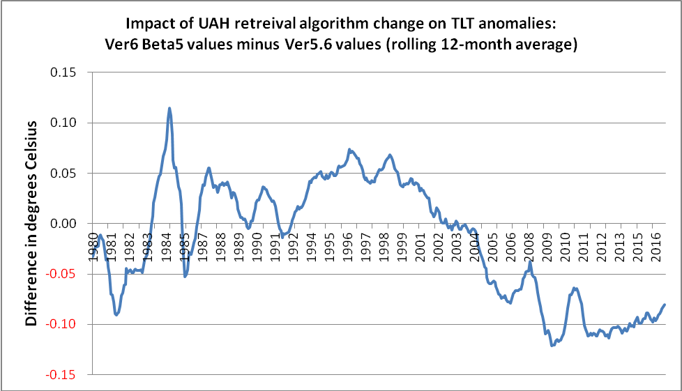
In terms of its impact on trend over the last 19 years or so, an obvious feature of the version change is that it boosts global temperatures in 1998 by just over 0.06° C, whilst lowering current temperatures by just over 0.08° C. Therefore, the net effect is to raise 1998 temperatures by about 0.15° C relative to today’s values. That is why some people refer to a mere 0.02° C difference between 1998 and 2016, whereas, NOAA NCEI shows this as 0.17° C.
(It is not difficult to imagine the hue and cry that would have gone up if one of the other datasets, such as NASA Gistemp, NOAA’s own Global Land & Ocean anomalies or the UK’s HadCRUT, had had a similar adjustment, but in the opposite direction.)
Anyway, it seemed pretty obvious which variant would have been used, so the task was merely to establish the exact start point. It transpires that if one ignores all the data before January 1998, and then superimposes a linear trend line, one does indeed get an R² value of ~ 0.019, as mentioned in one of the Tweets above. (The meaning of an R² value, as well as its use and misuse, will be discussed later in this piece.) In the interim, here is the chart…
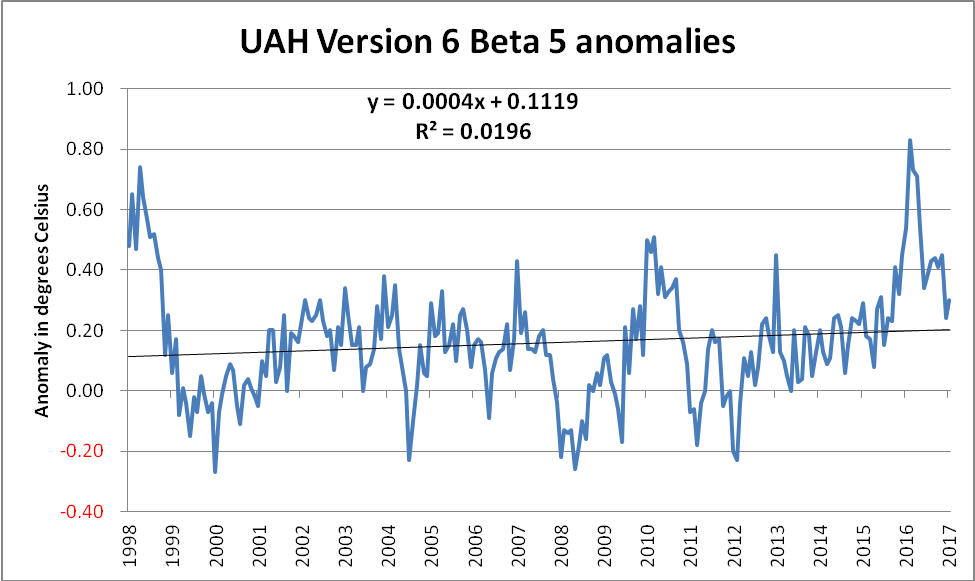
Those with some skill in dealing with such charts will recognise the gradient in the equation of the linear trend line,
Y = 0.0004X + 0.1119
As the data series is in terms of monthly anomalies, this value needs to be multiplied by 120 in order to convert it to the more familiar decadal trend form of +0.048° C/decade. Whilst this is certainly less than the trend using the full set of data, namely +0.123° C/decade, it is most assuredly non-zero.
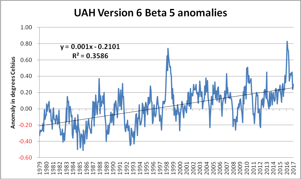
The full dataset (shown below) gives a far more complete picture, as well as demonstrating just how egregious the selection of the start point had been. Additionally, this also highlights just how much of an outlier the 1998 spike represents. Compare the size of the upward 1998 spike with the less impressive downward excursion shown around 1991/92. This downward excursion was caused by the spectacular Mt Pinatubo eruption(s) in June 1991. The Pinatubo eruption(s) did indeed have a temporary effect upon the planet’s energy imbalance, owing, in no small measure, to the increase in planetary albedo caused by the ~ 20 million tons of sulphur dioxide blasted into the stratosphere. On the other hand, the 1997/98 El Nino was more of an energy-redistribution between the ocean and the atmosphere. (The distinction between these types of event is sadly lost on some.)
The approach whereby inconvenient chunks of a dataset are conveniently ignored is a cherry-picking technique known as “end point selection”. It can also be used to actually identify those areas of the data which are most in line with the “climate change is a hoax” narrative. Once again, it is extremely easy to identify such regions of the data. A simple technique is to calculate the trend from every single starting date up until the present, and to then only focus on those which match the narrative. Doing this for the above dataset gives the following chart…
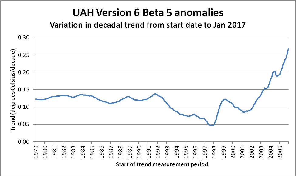
It can clearly be seen that the trend value becomes increasingly stable (at ~ +0.12° C/decade) as one utilises more and more of the available data. The trend also clearly reaches a low point – albeit briefly – at 1998. This is entirely due to the impact that the massive 1997/98 El Nino had on global temperatures – in particular on satellite derived temperatures.
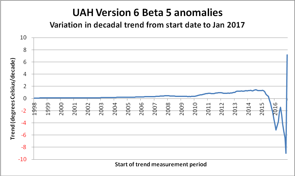
The observant reader will have undoubtedly noticed that the above chart ends at ~ 2006. The reason is simply because trend measurements become increasingly unstable as the length of the measurement period shortens. Not only do “short” trend values become extreme and meaningless, they also serve to compress the scale in areas of genuine interest. To demonstrate, here is the remainder of the data. Note the difference in the scale of the Y-axis…
Now, what about this thing referred to as the R² value? It is also known as the Coefficient of Determination, and can be a trap for the unwary. First of all, what does it actually mean? One description reads as follows…
It is a statistic used in the context of statistical models whose main purpose is either the prediction of future outcomes or the testing of hypotheses, on the basis of other related information. It provides a measure of how well observed outcomes are replicated by the model, based on the proportion of total variation of outcomes explained by the model.
In their online statistics course, Penn State feel obliged to offer the following warning…
Unfortunately, the coefficient of determination r² and the correlation coefficient r have to be the most often misused and misunderstood measures in the field of statistics.
…
The coefficient of determination r² and the correlation coefficient r quantify the strength of a linear relationship. It is possible that r² = 0% and r = 0, suggesting there is no linear relation between x and y, and yet a perfect curved (or “curvilinear” relationship) exists.
Here is an example of what that means. Consider a data series in which the dependent variable is comprised of two distinct signals. The first of these is a pure Sine-wave and the second is a slowly rising perfectly linear function.
The formula I used to create such a beast was simply… Y = SinX + 0.00005X (where x is simply angular degrees)
The chart, with its accompanying R² value, is shown below, and, coincidentally, does indeed bear quite a striking resemblance to the Keeling Curve…
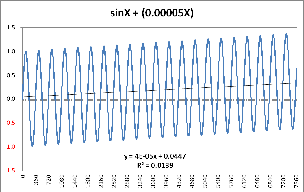
The function displayed is 100% predictable in its nature, and therefore it would be easy to project this further along the X-axis with 100% certainty of the prediction. If one were to select ANY point on the curve, moving one complete cycle to the right would result in the Y-value incrementing by EXACTLY +0.018 (360 degrees x 0.00005 = 0.018 per cycle). A similar single-cycle displacement to the left would result in a -0.018 change in the Y-value. In other words, the pattern is entirely deterministic. Despite this, the R² value is only 0.0139 – considerably less than the value of 0.0196 derived from the UAH data.
(NB There is a subtlety in the gradient which might require explanation. Although the generating formula clearly adds 0.00005 for each degree, the graph shows this as 0.00004 – or, more accurately as 0.000038. The reason is because the Sine function itself introduces a slight negative bias. Even after 21 full cycles, this bias is still -0.000012. Intuitively, one can visualise this as being due to the fact that the Sine function is positive over the 0 – 180 degree range, but then goes negative for the second half of each cycle. As the number of complete cycles rises, this bias tends towards zero. However, when one is working with such functions in earnest, this “seasonal” bias would have to be removed.)
Summing this up, trying to fit a linear trend to the simple (sine + ramp) function is certain to produce an extremely low R² value, as, except for the two crossover points each cycle, the difference between the actual value and the trend leaves large unaccounted-for residuals. To be in any way surprised by such an outcome is roughly akin to being surprised that London has more daylight hours in June than it does in December.
So what is the paradox with the low R² value for the UAH data? There isn’t one. Just as it would be daft to expect a linear trend line to map onto the future outcomes on the simple (sine + ramp) graph above, it would be equally daft to expect a linear trend line to be in any way an accurate predictor for the UAH monthly anomalies over the months and years to come.
Nevertheless, even although a linear trend produces such a low R² value when applied to the (sine + ramp), how does it fare as regards calculating the actual trend? Once the “seasonal” bias introduced by the presence of the sine function is removed, the calculated trend is EXACTLY equal to the actual trend embedded in the generating function.
Anyway, even if the period from January 1998 until January 2017 did indeed comprise the entirety of the available data, why would anyone try to use a linear trend line? If someone genuinely believed that the mere fact of a relatively higher R² value provided a better predictor, then surely that person might play around with some of the other types of trend line instantly available to anyone with Excel? (Indeed, any application possessing even rudimentary charting features would be suitable.) For example, a far better fit to the data is obtained by using a 5th order polynomial trend line, as shown below…
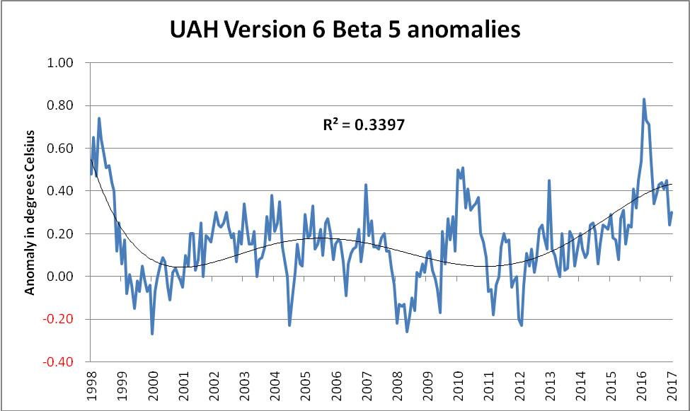
Although this is something of a “curve fitting” exercise, it seems difficult to argue with the case that this polynomial trend line looks a far better “fit” to the data than the simplistic linear trend. So, when someone strenuously claims that a linear trend line applied to a noisy dataset producing an R² value of 0.0196 means there had been no warming, then there are some questions which need to be asked and adequately answered:
Does that person genuinely not know what they’re talking about, or is their intention to deliberately mislead? (NB It should be obvious that these two options are not mutually exclusive, and therefore both could apply.)
Given that measurements of surface temperature, oceanic heat content, sea level rise, glacial mass balance, ice-sheet mass balance, sea ice coverage and multiple studies from the field of phenology all confirm global warming, why, one wonders, would somebody concentrate on an egregiously selected subset of a single carefully selected variant of a single carefully selected dataset?
You’re a credit to the internet, Jim: nice work.
You are very kind SML, but Bill deserves the credit for this one. All I did was scribble the intro!
Kudos to Bill the Frog then!
Nice work; a bit technical for this layperson, but I like to see the homework on display. It’s annoying that the overwhelming evidence of every kind and the scientific agreement are still being set aside. Nice point about lack of understanding and intent to mislead possibly overlapping.
Thanks Susan,
I will pass your kind words on to Bill at the earliest opportunity.
For a related, and highly topical, example of “lack of understanding and intent to mislead possibly overlapping” please see:
The House Science Climate Model Show Trial